Abstract

The debate covering stock return predictability is now shifted towards the investigation of changing patterns of return predictability as suggested by the adaptive market hypothesis (AMH). The present article inspects the varying return predictability pertaining to the equity market in Pakistan under AMH framework.  A nonlinear autoregressive neural network (NARNN) model is employed to investigate the nonlinear dependency of returns over a period of eighteen years. NARNN is a robust and flexible technique that is free from any restrictive assumptions. Under a rolling window framework, the repeating patterns of predictability and unpredictability are observed. This finding confirms the idea of AMH.

Key Words

Adaptive Market Hypothesis, Efficient Market Hypothesis, Artificial Neural Network,

                          Rolling Window Analysis

Introduction

The neoclassical thoughts of finance ignore the behavioral aspects of decision making. It demands homogeneity in participant’s beliefs while in practice the investor’s decisions have psychological effects. The behavioral school criticizes the traditional finance on the basis of psychological factors which they ignored and provided a new interaction between financial activity and psychology Fromlet (2001).  The emerging field of behavioral finance which brings the most contradictory research findings makes the validity of efficient market hypothesis (EMH) uncertain (Kahneman & Tversky (1979), Grossman & Stiglitz (1980), De Bondt & Thaler (1985).  Shlifer (2000) critically reviews the three main assumptions of EMH and argues that in real-world situations the decisions of irrational investors are based on the perception framed by them, the price fluctuations are attributed to underreaction and overreaction of the market participants and arbitrage opportunity is risky and limited. 

Traditionally the level of market efficiency was examined for some predetermined sample period (Campbell et al., 1997). The static approach of efficiency was easy to judge and this approach tells that the weather market is efficient or market is not efficient over the entire sample period. The viewpoint on the traditional focus of absolute, static and short-horizon predictability of EMH is now relocating and the time-varying  degree of efficiency is taking place over them  Campbell et al., (1997), Lo & MacKinlay (2002) and Lo (2008).  

The reconciliation approach of Lo (2004, 2005) brings the unique hypothesis introduced with the adaptive market hypothesis (AMH). The theories of traditional finance and behavioral finance are connected together through this hypothesis. It assumes that the efficiency level in a market remains to change and does not remain static. Arrival of new players, change in level of competition, different economic and political situations  and the  ability of investors  to adapt the new market conditions causes the change in level of efficiency in the market Kim et al., (2011).  Under an AMH framework the profit opportunities do exist on varying time period and market may be efficient on some times and inefficient on some other times Lim et al., (2013) and Urquhart and Mc Groarty (2014). 

Aforementioned theory of AMH is in its formative stage and only limited number of research studies available which empirically investigated its implications.  Underneath the AMH point of view, the nonlinear dependency of return over changing time period is desirable to detect. Only employing linear test to detect dependency is not sufficient as the nonlinear dependencies are still possible to exist if no dependency is suggested by linear techniques   Hiremath & Kamaiah (2010), Alagidede (2011), Caraiani (2012) Urquhart & Hudson (2013). Literature characterized the emerging economies as non-linear in terms of their stock prices movement Todea (2009).  Hinich & Patterson (2005) investigated the nonlinear dependency by using non-overlapped moving time windows on equally divided length of sample periods.

 These studies modeled the pattern of return predictability through traditional statistical techniques. Traditional statistical techniques are criticizes due to the imposed restriction on the data while using it for forecasting and for not being able to correctly model some complex nonlinear relationship. The Artificial neural networks (ANN) having the ability to learn complex relationships between variables, provide an alternative to overcome the shortcomings of conventional techniques to model the return predictability (Oliveira et al 2011, Maqaleh et al 2016 ).  ANNs gained wide attention in the domain of financial time series forecasting due to their nonlinear, nonparametric, self-adaptive and noise-tolerant properties Hussain et al., (2008), Khashei & Bijari (2010).  As compared to other linear and nonlinear statistical techniques, the ANN technique is consider more accurate to model a time series having  more nonlinearities  Lee & Chen (2005). ANNs with their inherent capabilities to identify any nonlinear complex relationship present in time series are being widely used in stock return prediction Dase & Pawar (2010). 

For an informationally inefficient stock market of Pakistan Haque et al (2011), Nisar, S., & Hanif, M. (2012) and with highly volatile economic condition, it is highly relevant to investigate the implications of AMH in Pakistan financial market. Urquhart & McGoarty (2016) in accordance to the proposed framework of AMH discover the direct relationship between fluctuating market situation and the ability to forecast the market. Possibility to predict the expected returns over different time periods relates to the different market conditions Noda (2016). And each and every market is characterized by dynamic market conditions so there is a need to evaluate each market individually based on unique circumstances. For evaluation such dynamic financial market one need to follow a dynamic procedure. There is a need to explore the complex relation of return predictability over varying time periods and different market conditions in Pakistan financial market. Therefore to explore the validity of AMH, in explaining the stock behavior over a long interval, the present study is conducted. By having the ability to model complex nonlinear relationship between variables applying ANN can we able to assess the implications of AMH in Pakistan financial market.  

Data 

The monthly return data of bench market index of Pakistan Stock Exchange (PSX) that is KSE-100 is taken as data sample for this study.  The sample period is comprises on data from January 2000 to December 2018. The sample period is taken due to the reasons because to make the study up to date by including current data in the article and this large data set will enable us to produce workable results by ensuring adequate data for rolling window analysis. It will also cover the most of the major events of Pakistan stock exchange and other economic and political events relevant to stock market functioning.  

Methodology

The methodology of the study is comprises on two stages. The first stage involves the steps to choose an optimal neural network model. At this stage the parameters for the optimal model are selected. Selection of parameters is done by considering performance measure errors. All the parameters which are helpful in minimising the error term is consider for the optimal model.

 At second stage this optimal neural network model will be used for modelling return predictability pattern.  A nonlinear auto regressive neural network model is used under rolling window frame work. The rolling window analysis enables us to examine the pattern of predictability over the changing time period without any delay in time (Charles et al., 2012). By plotting the performance measure errors through rolling window analysis on time will give insights to the changing degree of predictability. These stages are discussed in detail in the next section.

First stage: steps for optimal selection of ANN Model 

For designing an optimal ANN model we follow the eight step process presented by Kaastra and Boyd (1996).   

Step I: Variable Selection 

This step involves the selection of dependent and independent variables. In this study dependent variable is the natural logarithm return of KSE-100 index. Return is calculated according to the annual continuous compounded rate for a mentioned time period Nisar & Hanif (2012). Simply, the index value at time ‘t’ is divided by index value at time ‘t-1’ and then the log of this value represents the return. This may be represented in the form of equation as follows:

Rt = ln( Pt / Pt-1 ) ……………….. (1)

Where, 

Rt = Return for time‘t’

Ln = Natural log

Pt = Current price for time‘t’

Pt-1 = previous price of time‘t-1’

A lagged series is an independent variable under univariate time series analysis and this independent variable is an input variable for ANN Model. The selection of best lagged series is based on the low performance measure produced by using that lagged series.  Frequency of data is monthly Index values which are being used in the study. 

Step 2: Data Collection

The required data is taken from the web site of Pakistan Stock Exchange; www.psx.com.pk. And the information regarding relevant events is collected from 

Step 3: Data Pre-Processing

Variable are not fed to ANN in raw form, but they need to be analysed and transformed before using. Logarithmic transformation of the variables is done to minimise the noise and flatten the distribution of the data to assist ANN in learning the relevant patterns.

Step 4: Training, Testing, and Validation Sets

Data set is needed to divide into three distinctive sets. The data split ratio followed by the study is presented in table

Table 1.

Layers	Nodes	Training set	Testing set	Validation set
1,2	2, 3,4,…., 50	60%	20%	20%
1,2	2, 3,4,…., 50	65%	15%	20%
1,2	2, 3,4,…., 50	70%	15%	15%
1,2	2,3,4,…., 50	75%	10%	15%
1,2	2, 3,4,…., 50	80%	10%	10%
1,2	2, 3,4,…., 50	85%	05%	10%
1,2	2, 3,4,…., 50	90%	05%	05%

From the above possible combination of data split ratio, the best combination of data split ratio is selected after trial.

Step 5: Neural Network Paradigms

This step involves the selection of parameters involved in making neural network architecture. Nonlinear autoregressive feed-forward artificial neural network having multi-layer perceptions in Matlab R2018a, which this study is going to employ as (Adebiyi et al., 2014; Zhang 2003) with little modifications.  Equation 1 explains the relationship among the output and the inputs using linear and nonlinear activation functions, of a multilayer fed-forward neural network.

where j (j = 0; 1; 2;:::;h) and ij (i = 0; 1; 2;:::;p; j = 1; 2;:::;h) are the model parameters often called the connection weights; p is the number of input nodes and h is the number of hidden nodes. F and G are hidden and output layer activation functions, respectively. For hidden and out-put layers the sigmoid and linear functions are given in Eqs. 2  and 3, respectively Zhang (2003),  Khashei & Bijari (2011).

F(x) = …………………… (2)

G(x) = x ………………………. (3)  

In financial time series forecasting the minimum number of hidden layer is recommended for optimal working, because by increasing the hidden layers it increases its complexity. In time series forecasting mostly a feed forward network with single hidden layer is used for modelling the data set Zangh (2003). From one and two layers the best performing layer will be selected.

Under trial and error method backward approach is followed to select hidden nodes Panchal and Panchal (2014). Starting from 50 nodes and moving backward for selecting best performing nod. From 50 nodes the best performing node is selected for optimal ANN model.

Step 6: Evaluation criteria

Three statistical performance evaluation measures Mean Absolute Error (MAE), Mean squared error (MSE) and Root mean square error (RMSE) are being used by this study  (Shamisi, et al., 2013).. These performance error statistics can be defined as follows:

MAE=  ………………………............ (4)           

MSE=  ……………………………..  (5)

RMSE =  …………………. (6)

Where R_t and are, respectively, the actual returns and forecasted returns, and N is the size of the testing dataset.  Forecasting errors needs to be less for forecasting accuracies for financial time series. The point at which the minimum MSE is reported will be selected as best lag point for each country.

Step 7: Neural Network Training

In this study feed-forward neural networks is trained using Levenberg-Marquardt   learning algorithm as used by Shayea (2017). Matlab software is used for training the network. Matlab use train lm function to updates weight and bias values according to Levenberg-Marquardt optimization. This function uses 100 maximum numbers of epochs to train the network. The output is determined through a non-linear activation function. The activation function is usually a logistic function that transforms the output to a number that is between 0 &1.

Step 8: Implementation

Nonlinear autoregressive neural network is implemented under the above selected parameters. This experiment helps us to select optimal model for further analyses. 

Second stage: Using Optimal Architecture under Rolling Window Analysis

After construction of best combination of hidden layers (x), nodes (y) and lags (z) the point which reports minimum errors the next step is to constitute rolling window. Rolling window will be using the estimation window of 36 months with one month rolling. The equation for feed forward artificial neural network for rolling window is:

 ……………......... (7)

The training data window should be optimal because, “If the minimum training window is too long the model will be slow to respond to state changes., If the training window is too short, the model may overreact to noise” (Arlot & Celisse 2010). 

Figure 1

Schematic Diagram of Rolling Window Analysis



The optimal length of 36 months moving window is created and tested. The use of moving window approach enables us to capture the certain trends over moving time periods. 

The movement of error term in response to market conditions is analysed according to the following rule. If the error term are high in some market the prediction level is low and market is little efficient in that position as compare to the points where the error term are low. These levels of predictability are due to the prevailing market condition. So different scenarios are given in the table which will help to explain the KSE 100 movement towards efficiency or inefficiency or it is providing a better explanation of adaptive market hypothesis by showing cyclical efficiency.  



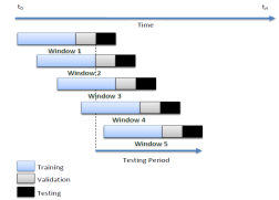
Figure 2

Movement of error term and levels of predictability



Empirical Results and Discussion

Descriptive statistics of the monthly return of the KSE-100 index show that the average monthly return at KSE-100 is 0.013879 with a standard deviation of 0.078258. The monthly return series is negatively skewed with a skewness value of -1.656 and a high value of kurtosis 13.747 which shows that distribution is not normal. The Jarque-Bera statistics for monthly return is 1175.235 and P- value is 0.0000 which shows that the daily return series does not follows normal distribution.

Table 3. Descriptive Statistics of KSE-100 Index Monthly Return

Statistics	KSE-100 Monthly return
Mean	0.013879
Standard deviation	0.078258
Skewness	-1.656
Kurtosis	13.747
Jarque–Bera	1175.235*

*denote significant at 1 % level

Results

Results of the study are divided in two stages as according to the described methodology. At the first stage the results for the selection of the optimal model for artificial neural network are presented. Nonlinear autoregressive neural network is run at different lags using fifty hidden neurons and at different combinations of data split ratio as of training, testing and validation set.  

Figures 3-6 reports the results of root mean square error at The arrival50 nodes for first four lags while using different combinations of data split ratios for training; testing and validation. A best combination of data split ratio which reports the lowest root mean square error, for each lag is selected from this exercise. .08,.15,.05, .70, .15, .15, .90,.05,.05 and .70, 10, 20 are the data split ratios which are showing lowest performance measure for the first, second, third and fourth lag respectively.    

Figure 3-6

RMSE-1, RMSE-2, RMSE-3 and RMSE-4 at different data split ratio



Above figures also provides valuable information about the number of nodes in the optimal model that by increasing the number of nodes in all combinations of data split ratios the value of performance error increases. The selection of nodes for the best combination of data split ratios is determined through the table 5-8. Table 5-8 reports the results of performance measure error at fifty nodes. The nodes at which the root mean square error is lowest are node 3, node 1, node 2 and node 4 for the first, second, third and fourth lag respectively.  So by keeping only lower number of hidden neuron we can have an optimal model for rolling window nonlinear auto regressive neural network in next stage.

Table 4. R MSE-1at node 1 to node 50

Comb/H.N	N1	N2	N3	N4	N5	N6	N7	N8
.6,.2,.2	0.0871429	0.0777065	0.0681314	0.0948506	0.08744	0.0723339	0.0804678	0.158522
.65, .15, .2	0.0875724	0.0777065	0.0662375	0.0962138	0.090858	0.0723339	0.0794958	0.158522
.65,.2,.15	0.0871429	0.0777065	0.0674325	0.0962138	0.08744	0.0723339	0.080145	0.158522
.7,.2,.1	0.0871429	0.0777065	0.0674325	0.0962138	0.090858	0.0723339	0.0794958	0.158522
.7,.15,.15	0.0878294	0.0777065	0.0662375	0.0962138	0.090858	0.0723339	0.0794958	0.158522
.7,.1,.2	0.0884779	0.0777322	0.0649009	0.0962138	0.0952367	0.0723339	0.0794958	0.158522
.75,.2,.05	0.0875724	0.0777065	0.0668866	0.0962138	0.090858	0.0723339	0.0794958	0.158522
.75,.15,.1	0.0882553	0.0777065	0.0662375	0.0962138	0.090858	0.0723339	0.0794958	0.158522
.75,.1,.15	0.0889562	0.0777322	0.0641353	0.0962138	0.0952367	0.0722395	0.0794958	0.158522
.75,.05,.2	0.0900455	0.077754	0.0633395	0.1086797	0.1079713	0.0709004	0.0775824	0.158522
.8,.05,.15	0.0904711	0.077754	0.0622665	0.1174934	0.1079713	0.069538	0.0775824	0.1845742
.8,.1,.1	0.0894551	0.0777322	0.0641353	0.1020115	0.1000195	0.0713379	0.0794958	0.158522
.8,.15,.05	0.0882553	0.0777065	0.0655928	0.0962138	0.0952367	0.0723339	0.0794958	0.158522
.85,.05,.1	0.0913187	0.077754	0.0623123	0.1300981	0.1176686	0.069538	0.0784604	0.1906585
.85,.1,.05	0.0894551	0.0777359	0.0641353	0.1020115	0.1000195	0.0709004	0.0788605	0.158522
.9,.05,.05	0.0925586	0.0777839	0.063988	0.1543938	0.1176686	0.0679255	0.0784604	0.2442362
Comb/H.N	N15	N20	N25	N30	N35	N40	N45	N50
.6,.2,.2	0.8540058	0.6168502	1.1183273	0.4948634	1.7217955	0.9181224	0.8662499	1.6956986
.65, .15, .2	0.8540058	0.6168502	1.1183273	0.4948634	1.7217955	0.9181224	0.8662499	1.6956986
.65,.2,.15	0.8540058	0.6168502	1.1183273	0.4948634	1.7217955	0.9181224	0.8662499	1.6956986
.7,.2,.1	0.8540058	0.6168502	1.1183273	0.4948634	1.7217955	0.9181224	0.8662499	1.6956986
.7,.15,.15	0.8540058	0.6168502	1.1183273	0.4948634	1.7217955	0.9181224	0.8662499	1.6956986
.7,.1,.2	0.8540058	0.6168502	1.1183273	0.4948634	1.7217955	0.9181224	0.8662499	1.6956986
.75,.2,.05	0.8540058	0.6168502	1.1183273	0.4948634	1.7217955	0.9181224	0.8662499	1.6956986
.75,.15,.1	0.8540058	0.6168502	1.1183273	0.4948634	1.7217955	0.9181224	0.8662499	1.6956986
.75,.1,.15	0.8540058	0.6168502	1.1183273	0.4948634	1.7217955	0.9181224	0.8662499	1.6956986
.75,.05,.2	0.8540058	0.6168502	1.1651408	0.4948634	1.7217955	0.9181224	0.8662499	1.6956986
.8,.05,.15	0.8540058	0.6168502	1.1651408	0.4948634	1.7217955	0.9181224	0.8662499	1.6956986
.8,.1,.1	0.8540058	0.6168502	1.1651408	0.4948634	1.7217955	0.9181224	0.8662499	1.6956986
.8,.15,.05	0.8540058	0.6168502	1.1183273	0.4948634	1.7217955	0.9181224	0.8662499	1.6956986
.85,.05,.1	0.8540058	0.6168502	1.1651408	0.4948634	1.7217955	0.9181224	1.2830719	1.6956986
.85,.1,.05	0.8540058	0.6168502	1.1651408	0.4948634	1.7217955	0.9181224	0.8662499	1.6956986
.9,.05,.05	0.8540058	0.6168502	1.1651408	0.4948634	1.7217955	0.9181224	1.2830719	1.6956986

Table 5. R MSE-2at node 1 to node 5

Comb/H.N	N1	N2	N3	N4	N5	N6	N7	N8
.6,.2,.2	0.076488	0.08083	0.080475	0.080454	0.077759	0.082688	0.088633	0.077956
.65,.15,.2	0.076459	0.081464	0.081179	0.080789	0.078423	0.082599	0.090661	0.078178
.65,.2,.15	0.076623	0.081223	0.080475	0.080454	0.077759	0.082599	0.090661	0.077956
.7,.2,.1	0.076459	0.08133	0.080475	0.080454	0.078038	0.082599	0.090661	0.077956
.7,.15,.15	0.076459	0.081464	0.081882	0.080832	0.078423	0.082692	0.090661	0.078558
.7,.1,.2	0.076506	0.081892	0.082999	0.08141	0.078423	0.082857	0.09079	0.078278
.75,.2,.05	0.076459	0.081464	0.081087	0.080561	0.078423	0.082599	0.090661	0.078178
.75,.15,.1	0.076462	0.081892	0.081882	0.080975	0.078423	0.082748	0.090661	0.078278
.75,.1,.15	0.076467	0.08255	0.082999	0.082025	0.07906	0.082857	0.09079	0.078278
.75,.05,.2	0.076467	0.083644	0.08384	0.08268	0.083312	0.083106	0.099939	0.078579
.8,.05,.15	0.076552	0.084454	0.085112	0.084488	0.086542	0.083577	0.099939	0.079257
.8,.1,.1	0.076467	0.08255	0.08384	0.08268	0.079995	0.083106	0.094729	0.078404
.8,.15,.05	0.076462	0.081892	0.082999	0.080975	0.078423	0.082857	0.090661	0.078278
.85,.05,.1	0.076552	0.085593	0.085112	0.084488	0.091624	0.084625	0.103356	0.079257
.85,.1,.05	0.076467	0.082927	0.08384	0.08268	0.081217	0.083106	0.094729	0.078579
.9,.05,.05	0.076987	0.087791	0.08744	0.088327	0.101376	0.100363	0.103356	0.086524
Comb/H.N	N15	N20	N25	N30	N35	N40	N45	N50
.6,.2,.2	0.329589	0.809611	1.010588	0.365689	0.666941	0.675425	0.990145	1.742632
.65, .15, .2	0.329589	0.809611	1.010588	0.365689	0.666941	0.675425	0.990145	1.742632
.65,.2,.15	0.329589	0.809611	1.010588	0.365689	0.666941	0.675425	0.990145	1.742632
.7,.2,.1	0.329589	0.809611	1.010588	0.365689	0.666941	0.675425	0.990145	1.742632
.7,.15,.15	0.329589	0.809611	1.010588	0.365689	0.666941	0.675425	0.990145	1.742632
.7,.1,.2	0.329589	0.809611	1.010588	0.306386	0.666941	0.675425	0.990145	1.742632
.75,.2,.05	0.329589	0.809611	1.010588	0.365689	0.666941	0.675425	0.990145	1.742632
.75,.15,.1	0.329589	0.809611	1.010588	0.365689	0.666941	0.675425	0.990145	1.742632
.75,.1,.15	0.318707	0.809611	1.010588	0.306988	0.666941	0.675425	0.990145	1.742632
.75,.05,.2	0.330477	0.809611	1.010588	0.365818	0.666941	0.675425	0.990145	1.742632
.8,.05,.15	0.34309	0.809611	1.010588	0.365818	0.666941	0.675425	0.990145	1.742632
.8,.1,.1	0.318707	0.809611	1.010588	0.306988	0.666941	0.675425	0.990145	1.742632
.8,.15,.05	0.329589	0.809611	1.010588	0.306386	0.666941	0.675425	0.990145	1.742632
.85,.05,.1	0.34911	0.809611	1.010588	0.365818	0.666941	0.675425	0.990145	1.742632
.85,.1,.05	0.321971	0.809611	1.010588	0.365818	0.666941	0.675425	0.990145	1.742632
.9,.05,.05	0.34911	0.809611	1.010588	0.365818	0.666941	0.675425	0.990145	1.742632

Table 6. R MSE-3 at node 1 to node 50

Comb/H.N	N1	N2	N3	N4	N5	N6	N7	N8
.6,.2,.2	0.078692	0.077616	0.07873	0.079196	0.081837	0.082009	0.081951	0.084031
.65, .15, .2	0.078763	0.077618	0.078708	0.079542	0.082142	0.083106	0.082582	0.084031
.65,.2,.15	0.078692	0.077629	0.078708	0.079196	0.081917	0.082009	0.08219	0.084031
.7,.2,.1	0.078715	0.077629	0.078708	0.079196	0.082142	0.082537	0.08219	0.084031
.7,.15,.15	0.078777	0.077618	0.078783	0.079542	0.082684	0.083106	0.083788	0.084896
.7,.1,.2	0.078777	0.077671	0.078958	0.080269	0.084078	0.083757	0.087859	0.087568
.75,.2,.05	0.078715	0.077629	0.078708	0.079196	0.082142	0.082537	0.08219	0.084031
.75,.15,.1	0.078777	0.077618	0.078947	0.079542	0.082917	0.083106	0.084939	0.086199
.75,.1,.15	0.07879	0.077587	0.079033	0.081136	0.084078	0.085188	0.087859	0.087568
.75,.05,.2	0.07879	0.077603	0.079033	0.081899	0.176237	0.087636	0.087859	0.090254
.8,.05,.15	0.07879	0.077564	0.079033	0.082995	0.222392	0.09185	0.090443	0.094965
.8,.1,.1	0.07879	0.077587	0.079033	0.081832	0.087906	0.085188	0.087859	0.087568
.8,.15,.05	0.078777	0.077556	0.078947	0.080269	0.082917	0.083106	0.086181	0.086199
.85,.05,.1	0.078846	0.077564	0.079622	0.084757	0.218313	0.101089	0.090443	0.102392
.85,.1,.05	0.07879	0.077604	0.079033	0.081832	0.087906	0.085188	0.087859	0.090254
.9,.05,.05	0.079304	0.077547	0.079964	0.084757	0.21555	0.101089	0.092693	0.119395
Comb/H.N	N15	N20	N25	N30	N35	N40	N45	N50
.6,.2,.2	0.224166	0.581126	0.649279	0.780372	1.076284	0.658626	1.105486	1.583643
.65, .15, .2	0.236535	0.581126	0.649279	0.780372	1.076284	0.652432	1.105486	1.583643
.65,.2,.15	0.224166	0.581126	0.649279	0.780372	1.076284	0.658626	1.105486	1.583643
.7,.2,.1	0.224166	0.581126	0.649279	0.780372	1.076284	0.658626	1.105486	1.583643
.7,.15,.15	0.22791	0.581126	0.649279	0.780372	1.076284	0.652432	1.105486	1.583643
.7,.1,.2	0.226902	0.581126	0.628242	0.780372	1.076284	0.694743	1.105486	1.583643
.75,.2,.05	0.224166	0.581126	0.649279	0.780372	1.076284	0.658626	1.105486	1.583643
.75,.15,.1	0.229767	0.581126	0.649279	0.780372	1.076284	0.652432	1.105486	1.583643
.75,.1,.15	0.22998	0.581126	0.628242	0.780372	1.076284	0.694743	1.105486	1.583643
.75,.05,.2	0.238733	0.581126	0.668724	0.780372	1.076284	0.727426	1.105486	1.583643
.8,.05,.15	0.238733	0.63271	0.668724	0.780372	1.076284	0.727426	1.105486	1.583643
.8,.1,.1	0.230094	0.581126	0.594439	0.780372	1.076284	0.694743	1.105486	1.583643
.8,.15,.05	0.226902	0.581126	0.628242	0.780372	1.076284	0.672239	1.105486	1.583643
.85,.05,.1	0.240567	0.63271	0.702359	0.853942	1.076284	0.741446	1.105486	1.583643
.85,.1,.05	0.233305	0.581126	0.594439	0.780372	1.076284	0.727426	1.105486	1.583643
.9,.05,.05	0.240675	0.63271	0.702359	0.853942	1.141387	0.743971	1.105486	1.583643

Table 7. R MSE-3 at node 1 to node 50

Comb/H.N	N1	N2	N3	N4	N5	N6	N7	N8
.6,.2,.2	0.078881	0.077755	0.080605	0.077593	0.081087	0.132182	0.083044	0.082383
.65, .15, .2	0.080061	0.07777	0.080993	0.077945	0.085759	0.132182	0.083439	0.082383
.65,.2,.15	0.078881	0.077755	0.080699	0.077593	0.081796	0.132182	0.083439	0.082383
.7,.2,.1	0.079361	0.07777	0.080699	0.077593	0.081796	0.132182	0.083439	0.082383
.7,.15,.15	0.080061	0.07777	0.080993	0.077945	0.085759	0.132182	0.084693	0.082383
.7,.1,.2	0.081031	0.077755	0.08124	0.078455	0.085759	0.132182	0.085809	0.083516
.75,.2,.05	0.079361	0.07777	0.080882	0.077945	0.083213	0.132182	0.083439	0.082383
.75,.15,.1	0.080061	0.077755	0.08124	0.078031	0.085759	0.132182	0.084693	0.082383
.75,.1,.15	0.082619	0.077755	0.081532	0.078835	0.085759	0.132182	0.085809	0.083516
.75,.05,.2	0.084571	0.077755	0.082224	0.079838	0.09076	0.132182	0.090362	0.092941
.8,.05,.15	0.088195	0.077755	0.08237	0.081885	0.09076	0.132182	0.095644	0.092941
.8,.1,.1	0.082619	0.077755	0.081765	0.079116	0.089927	0.132182	0.087268	0.085545
.8,.15,.05	0.082619	0.077755	0.081765	0.079116	0.089927	0.132182	0.087268	0.085545
.85,.05,.1	0.088195	0.077765	0.082595	0.085051	0.096161	0.132182	0.103502	0.092941
.85,.1,.05	0.088195	0.077765	0.082595	0.085051	0.096161	0.132182	0.103502	0.092941
.9,.05,.05	0.10324	0.077763	0.082669	0.092433	0.097842	0.132182	0.118835	0.102265
Comb/H.N	N15	N20	N25	N30	N35	N40	N45	N50
.6,.2,.2	0.132588	1.367142	1.341733	0.476854	1.738251	0.9577	0.742921	0.967878
.65, .15, .2	0.132588	1.367142	1.341733	0.476854	1.738251	0.9577	0.742921	0.967878
.65,.2,.15	0.132588	1.367142	1.341733	0.476854	1.738251	0.9577	0.742921	0.967878
.7,.2,.1	0.132588	1.367142	1.341733	0.476854	1.738251	0.9577	0.742921	0.967878
.7,.15,.15	0.130603	1.367142	1.341733	0.476854	1.738251	0.9577	0.742921	0.967878
.7,.1,.2	0.192835	1.367142	1.341733	0.476854	1.738251	0.9577	0.742921	0.967878
.75,.2,.05	0.132588	1.367142	1.341733	0.476854	1.738251	0.9577	0.742921	0.967878
.75,.15,.1	0.178954	1.367142	1.341733	0.476854	1.738251	0.9577	0.742921	0.967878
.75,.1,.15	0.331235	1.367142	1.341733	0.476854	1.738251	0.9577	0.742921	0.967878
.75,.05,.2	0.719118	1.367142	1.341733	0.476854	1.738251	0.9577	0.91157	0.967878
.8,.05,.15	0.576865	1.367142	1.341733	0.476854	1.738251	0.9577	0.91157	0.967878
.8,.1,.1	0.474361	1.367142	1.341733	0.476854	1.738251	0.9577	0.742921	0.967878
.8,.15,.05	0.474361	1.367142	1.341733	0.476854	1.738251	0.9577	0.742921	0.967878
.85,.05,.1	0.636563	1.367142	1.341733	0.476854	1.738251	0.9577	0.91157	0.967878
.85,.1,.05	0.636563	1.367142	1.341733	0.476854	1.738251	0.9577	0.91157	0.967878
.9,.05,.05	0.656375	1.367142	1.341733	0.476854	1.738251	1.355673	0.91157	0.967878

Table 4-7.  RMSE-1, RMSE-2, RMSE-3 and RMSE-4 at fifty nodes

From the above experiment we come to know about the optimal parameters which are reporting lowest root mean square error for all four lags.  The next step reports the non linear autoregressive rolling window analysis by using these optimal parameters for model construction for all four lags. The selected optimal parameters are used to run rolling window non-liner autoregressive neural network.  From this rolling analysis the lag series  which  report the lowest root mean square error will be selected as best lag for further analysis.

Non linear auto regressive neural network rolling window analysis

This second stage reports the results of performance measure errors through NAR neural network under rolling window analysis. A thirty six month rolling window is taken to run NAR neural network on all the four lags by using optimal parameters selected in the previous stage.  The optimal models to run rolling window analysis for the four lags are reported in table 8.  

Table 8. Optimal parameters

Lag	Training ratio	Testing ratio	Validation ratio	Nodes	Layers	Window size
First lag	80	15	05	03	1	36
Second lag	70	15	15	1	1	36
Third lag	90	05	05	02	1	36
Fourth lag	70	10	20	04	1	36

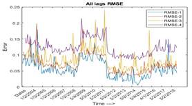
The rolling window analysis enables us to capture the variations in stock return predictability. Rolling window analysis also proves that the chances of predictability is high at lag one, as the lags values are increased the forecasting ability of the market start vanishing. As shown in figure 6 the rolling root mean square error is moving upward as with the increase of lag value.  This observation might mean that all the information is absorbed by the market after one month of trading. From this analysis we can chose lag one as the best lag for further analysis. 

It is apparent in the figure 6 that the rolling root mean square error of all four lags is moving in cyclical fashion.   It elucidate that a cyclical fashion changing degree of efficiency is observed and there are periods in where the market is more efficient than others (Urquhart & McGroarty 2016).  The low level of performance measuring errors shows that the forecasting error is least and it’s relatively easy to forecast the return opportunities in these time periods. And the time periods, in which performance measuring errors are higher, it’s difficult to forecast the market. However EMH theory does not explain such cycles (Lo, 2005).

Figure 7 and 8

RMSE all lags and threshold point



Lag one is showing the lowest root mean square error so by introducing a threshold point on the performance measure errors of lag one captured thorough 36 months rolling window the picture becomes clearer. When the performance measure error is less than 0.05 it shows that the index was predictable at that time and can be concluded as week form inefficient. Figure 7 exhibits the movement of performance error against the .05 threshold point.

Table 9. Degree of predictability

Time period	Performance measure error	Rejection /acceptance
Feb03-Dec04	Large RMSE	rejection
Jan05-Feb09	Low RMSE	acceptance
Jan09-Nov11	High RMSE	rejection
Dec11-April16	Low RMSE	acceptance
May16-Dec18	Mix outcome	Mix outcome

Table 9 reports the periods of predictability and no predictability. The period which is showing the high-performance measure error is rejecting the possibility for prediction. And the periods with low-performance measure error representing the time period in which there is no possibility to predict the future return. These patterns of predictability and no predictability are consistent with the findings of Kim et al. (2011), Alvarez-Ramirez et al. (2012), Urquhart and Hudson (2013), Noda (2016). It indicates that the markets follow the learning process, they learn from the environment and adapt accordingly. Markets are dependent on changing market conditions. 

Conclusion

This paper examines the degree of return predictability in the Pakistan stock market to test the new proposed framework of the adaptive market hypothesis. The monthly returns of the KSE-100 index from January 2000 to December 2018 are selected to investigate the changing patterns of return predictability. The degree of return predictability is measured by the nonlinear autoregressive neural network under the rolling window framework. In the two-stage methodology first, the parameters are selected for the optimal model on the bases of the lowest performance measure error. Selected parameters are used to model the optimal structure of the nonlinear autoregressive neural network model. 

In the second stage, the rolling nonlinear autoregressive neural network analysis is conducted. This analysis is used to track the time-varying efficiency and inefficiency consistent with AMH. The rolling window analysis is helpful to fully cover the dynamics of time series.  The results indicate that there are some periods in which the Pakistan stock market is showing a low level of predictability than others where the index is not predictable. This observation is consistent with AMH's evolving view of market efficiency.

The changing nature of predictability can further be elaborated by considering the market dynamics. Every market has its own characteristics on which its level of predictability is dependent. 

Figure 2-a



Figure 2-b



Figure 3-a



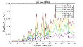
Figure 3-b



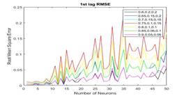
Figure 3-c



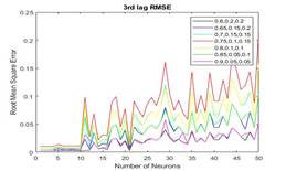
Figure 3-d



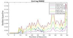
Figure 7



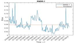
Figure 8

References

• Adebiyi, A. A., Adewumi, A. O., & Ayo, C. K. (2014). Comparison of ARIMA and artificial neural networks models for stock price prediction.Journal of Applied Mathematics,2014
• Alagidede, P. (2011). Return behaviour in Africa's emerging equity markets.The Quarterly Review of Economics and Finance,51(2), 133-140
• Al-Maqaleh, B. M., Al-Mansoub, A. A., & Al-Badani, F. N. (2016). Forecasting using artificial neural network and statistics models.International Journal of Education and Management Engineering,6(3), 20-32
• Al-Shamisi, M. H., Assi, A. H., & Hejase, H. A. (2013). Artificial neural networks for predicting global solar radiation in Al Ain city-UAE.International journal of green energy,10(5), 443-456
• Al-Shayea, Q. (2017). Neural Networks to Predict Stock Market Price. InWorld Congress on Engineering and Computer Science, San Fransisco(pp. 1-7
• Alvarez-Ramirez, J., Rodriguez, E., & Espinosa-Paredes, G. (2012). Is the US stock market becoming weakly efficient over time? Evidence from 80-year-long data.Physica A: Statistical Mechanics and its Applications,391(22), 5643-5647
• Arlot, S., & Celisse, A. (2010). A survey of cross-validation procedures for model selection.Statistics surveys,4, 40-79
• Campbell, J. Y., Champbell, J. J., Campbell, J. W., Lo, A. W., Lo, A. W., & MacKinlay, A. C. (1997).The econometrics of financial markets. princeton University press
• Caraiani, P. (2012). Characterizing emerging European stock markets through complex networks: From local properties to self-similar characteristics.Physica A: Statistical Mechanics and its Applications,391(13), 3629-3637.
• Charles, A., Darné, O., & Kim, J. H. (2012). Exchange-rate return predictability and the adaptive markets hypothesis: Evidence from major foreign exchange rates.Journal of International Money and Finance,31(6), 1607-1626
• Dase, R. K., & Pawar, D. D. (2010). Application of Artificial Neural Network for stock market predictions: A review of literature.International Journal of Machine Intelligence,2(2), 14-17
• De Bondt, W. F., & Thaler, R. (1985). Does the stock market overreact?.The Journal of finance,40(3), 793-805.de Oliveira, F. A., Zárate, L. E., de Azevedo Reis, M., & Nobre, C. N. (2011, October). The use of artificial neural networks in the analysisand prediction of stock prices. In2011 IEEE International Conference on Systems, Man, and Cybernetics(pp. 2151-2155). IEEE
• Fromlet, H. (2001). Behavioral finance-theory and practical application: Systematic analysis of departures from the homo oeconomicus paradigm are essential for realistic financial research and analysis.Business economics, 63-69
• economics, 63-69.Grossman, S. J., & Stiglitz, J. E. (1980). On the impossibility of informationally efficient markets.The American economic review,70(3), 393-408
• Haque, A., Liu, H.-C., & Fakhar-Un-Nisa. (2011). Testing the Weak Form Efficiency of Pakistani Stock Market (2000-2010). International Journal of Economics and Financial Issues , 1 (4), 153-162
• Hinich, M. J., & Patterson, D. M. (2005). Detecting epochs of transient dependence in white noise, Money, Measurement and Computation.edited by M. Belongia and J. Binner, London.
• Hiremath, G. S., & Kamaiah, B. (2010). Non-linear dependence in stock returns: Evidences from India.Journal of Quantitative Economics,8(1)
• Hussain, A. J., Knowles, A., Lisboa, P. J., & El-Deredy, W. (2008). Financial time series prediction using polynomial pipelined neural networks.Expert Systems with Applications,35(3), 1186-1199
• Kaastra, I., & Boyd, M. (1996). Designing a neural network for forecasting financial and economictime series.Neurocomputing,10(3), 215-236
• Kahneman, D. (1979). Tversky A.(1979).Prospect theory: an analysis of decision under risk, 263-292
• Khashei, M., & Bijari, M. (2010). An artificial neural network (p, d, q) model for timeseries forecasting.Expert Systems with applications,37(1), 479-489
• Khashei, M., & Bijari, M. (2011). A novel hybridization of artificial neural networks and ARIMA models for time series forecasting.Applied Soft Computing,11(2), 2664-2675
• Kim, J. H., Shamsuddin, A., & Lim, K. P. (2011). Stock return predictability and the adaptive markets hypothesis: Evidence from century-long U.S. data. Journal of Empirical Finance, 18(5), 868-879
• Lee, T. S., & Chen, I. F. (2005). A two-stage hybrid credit scoring model using artificial neural networks and multivariate adaptive regression splines. Expert Systems with Applications, 28(4), 743-752.
  http://dx.doi.org/10.1016/j.eswa.2004.12.031
• Lim, K. P., Luo, W., & Kim, J. H. (2013). Are US stock index returns predictable? Evidence from automatic autocorrelation-based tests.Applied Economics,45(8), 953-962.Lo, A. W. (2004). The adaptive markets hypothesis.The Journal of Portfolio Management,30(5), 15-29
• Lo, A. W. (2005). Reconciling efficient markets with behavioral finance: The adaptive markets hypothesis. Journal of Investment Consulting, 7(2), 21-44
• Lo, A. W., & MacKinlay, A. C. (2002).A non-random walk down Wall Street. Princeton University Press
• Nisar, S., & Hanif, M. (2012). Testing weak form of efficient market hypothesis: empirical evidence from South Asia.World Applied Sciences Journal,17(4), 414-427
• Noda, A. (2016). A test of the adaptive market hypothesis using a time-varying AR model in Japan.Finance Research Letters,17, 66-71
• Panchal, F. S., & Panchal, M. (2014). Review on methods of selecting number of hidden nodes in artificial neural network.International Journal of Computer Science and Mobile Computing,3(11), 455-464
• Shleifer, A. (2000).Inefficient markets: An introduction to behavioural finance. OUP Oxford.
• Todea, A., Ulici, M., & Silaghi, S. (2009). Adaptive markets hypothesis: Evidence from Asia-Pacific financial markets.The Review of Finance and Banking,1(1)
• Urquhart, A. and McGroarty, F. (2016) Are stock markets really efficient? Evidence of the adaptive market hypothesis, International Review of Financial Analysis, 47, 39-49.
• Urquhart, A., & Hudson, R. (2013). Efficient or adaptive markets? Evidence from major stock markets using very long run historic data.International Review of Financial Analysis,28, 130-142.
• Urquhart, A., & McGroarty, F. (2014). Calendar effects, market conditions and the Adaptive Market Hypothesis: Evidence from long-run US data.International Review of Financial Analysis,35, 154-166.
• Zhang, G. P. (2003). Time series forecasting using a hybrid ARIMA and neural network model.Neurocomputing,50, 159-175.
• Zhang, G. P., Patuwo, B. E., & Hu, M. Y. (2001). A simulation study of artificial neural networks for nonlinear time-series forecasting.Computers & Operations Research,28(4), 381-396